
UBMP4 Starter Project 1 - TV Remote
TV Remote Control Transmitter
The built-in infrared (IR) LED and pushbuttons make it easy to turn UBMP4 into a simple TV remote control transmitter. The programming knowledge needed to implement this functionality is relatively basic, too, giving you an opportunity to exercise all the skills introduced in the introductory programming activities on the website.
Don’t have a UBMP4? That’s ok, the explanations and code concepts introduced in this project will help you to code a TV remote transmitter program for other microcontroller devices, too. Specifically, this activity will lead you through the development and testing of functions to modulate data in the SONY SIRC (SONY IR Control) protocol. Afterwards, you will be able to apply this knowledge to modify the program so it can transmit data using other protocols such as NEC, Sharp, and the Philips RC-5 and RC-6 protocols – or even create your own protocols for your own projects!
This project will also demonstrate debugging techniques using both an oscilloscope, and the especially-useful code simulator built into the MPLAB X IDE. Before diving in, there are a few important concepts to know about how IR transmitters work and data modulation and encoding techniques they use. Let’s go!
How does a remote control transmitter work?
Most people reading this will already be aware that there is an LED at the top end of a TV remote, and will have hypothesized that the LED must somehow flash a coded signal to the TV to tell it what to do. Yet, it’s hard to prove this assumption by watching the LED, since all remote control transmitters use infrared (IR) light with a wavelength just outside of the visible spectrum to transmit their signals – meaning, we can’t see it. Still, being the inquisitive type, you probably blocked or obscured the LED at some point and, when nothing happened while you pressed the buttons, confirmed your intuition that the LED was indeed a necessary part of transmitting the control signals to the TV or device.

Whenever a button is pressed, an LED flashes behind the dark window of this TV remote. The flashes are barely visible because cameras contain an IR cut filter to block infrared light – but a little bit of light can still sneak through in the form of the dim flashing light right in the middle of the remote window.
Encoding data with light
How does the LED send its data? Knowing something about binary numbers, you might think it’s possible to use a simple transmission scheme in which turning the LED on represents a binary 1, while turning the LED off represents binary 0, and just having the LED flash out a sequence of ones and zeros makes binary codes. Unfortunately, there are (at least) two problems with this line of thought.
First, the light intensity of a battery operated remote transmitter is very low when compared with possible interference sources such as sunlight streaming through a window or, before we had more efficient LED lighting, incandescent light bulbs in the same room as the TV. The signal from the TV remote’s LED is just not powerful enough to overcome the interference from other potential IR sources.
The second problem is one of data encoding. Unlike using a wire in a closed circuit to carry current to a device, the space between a TV remote and its TV is open, and is therefore unreliable.
Here’s how to think about this problem. Say you had a closed circuit with a battery, a switch, and an LED. Turning on the switch allows current to flow to the LED, and lighting it up. The LED in the circuit clearly stays lit while the switch is on, so you can use the light coming from the LED as a reliable indicator of state – when it’s on, the light of the LED can represent a binary 1.
Conversely, when the switch is off, the current through the circuit is interrupted and the LED turns off. This also works consistently, so the absence of light can reliably represent a binary 0. It’s reliable because it always behaves the same way, and it behaves the same way because it’s in a closed circuit until something major changes – the switch breaking, or the battery dying, for example.
At first glance, using an LED to send data across the room to the TV might seem the same aw watching an LED in a circuit. You press a button the TV remote and its LED turns on, or flashes on an off. Even though you can’t see it, you know the LED must turn on at some points. The TV does have a receiver circuit that can see the LED, and if it sees the LED being on even when we cannot, why can’t it represent the light from the LED as a binary 1? Well, it can, but what if the LED is on, and your dog’s wagging tail blocks the signal between the remote control and the TV. The 1 now being transmitted by the remote will now be received as a 0 by the TV, because the dog’s wagging tail blocked the light and created interference. But don’t blame the dog! It’s not the dog’s fault – it’s just that the room, with the dog in it, is an unreliable medium in comparison to a closed circuit.
The solution to the problem involves finding a way to transmit both binary states, 0 and 1, by actively transmitting a signal for each state, instead of allowing one of those data states to simply be the absence of a signal. The light has to be on to be received as a 1, and the light has to be on to be received as a 0. Transmitting each signal using light (instead of dark) helps to make the signal reception more reliable, but now each of the two light signals need to be different from one another. And, both signals have to be transmitted using either more power, or by some other method to overcome the interference sources in the room. More power is difficult to achieve in a battery-operated remote, but a process known as modulation can be used to make the LED’s signal appear different enough from sunlight and room lights to work.
New Concepts
Infrared (IR) remote control systems modulate light beams to encode information. Here are some important concepts to learn:
Modulation - the process of mixing a data signal with another signal, called a carrier signal, in a way that the data can be extracted later by demodulation.
Demodulation - the process of recovering a data signal from a modulated signal.
Carrier - a known signal mixed with data to make it possible to transmit the data more reliably.
Frequency - the number of waves per second of an electronic signal (for our purposes), measured in Hz (Hertz)
Code - a digital representation of information. For example, each letter you see here is represented in your computer by a digital code (usually interpreted as a number).
Device/Address - a code representing the device being controlled
Command/Data - a code representing the command sent to the device
Pulse Width Modulation - encoding data using variable width pulses separated by spaces
Pulse Distance Modulation - encoding data using variable width spaces between fixed-length pulses
Bi-Phase Modulation (Manchester coding) - encoding data using opposite pairs of pulses and spaces (e.g. pulses then space for one state, and space then pulses for the opposite state)
Modulation and demodulation
Modulation is the process of combining a data signal with a carrier signal for the purpose of transmitting the data signal. Of course, after transmission, it’s important to be able to extract the data signal from the combined signal using a process known as demodulation.
To transmit light signals across a room, the carrier signal is often a rapidly pulsing light wave. Since sunlight is constant (or changes comparatively slowly in intensity, mostly due to clouds and weather, and to a much lesser extent time of day), and room lights flash at 60 Hz (in North America, and 50 Hz in many other locations), flashing an LED at a really rapid rate (usually 30-50 kHz) makes its signal different enough that it can be reliably detected despite the other interference sources – except for the dog, but we’ll get to that.
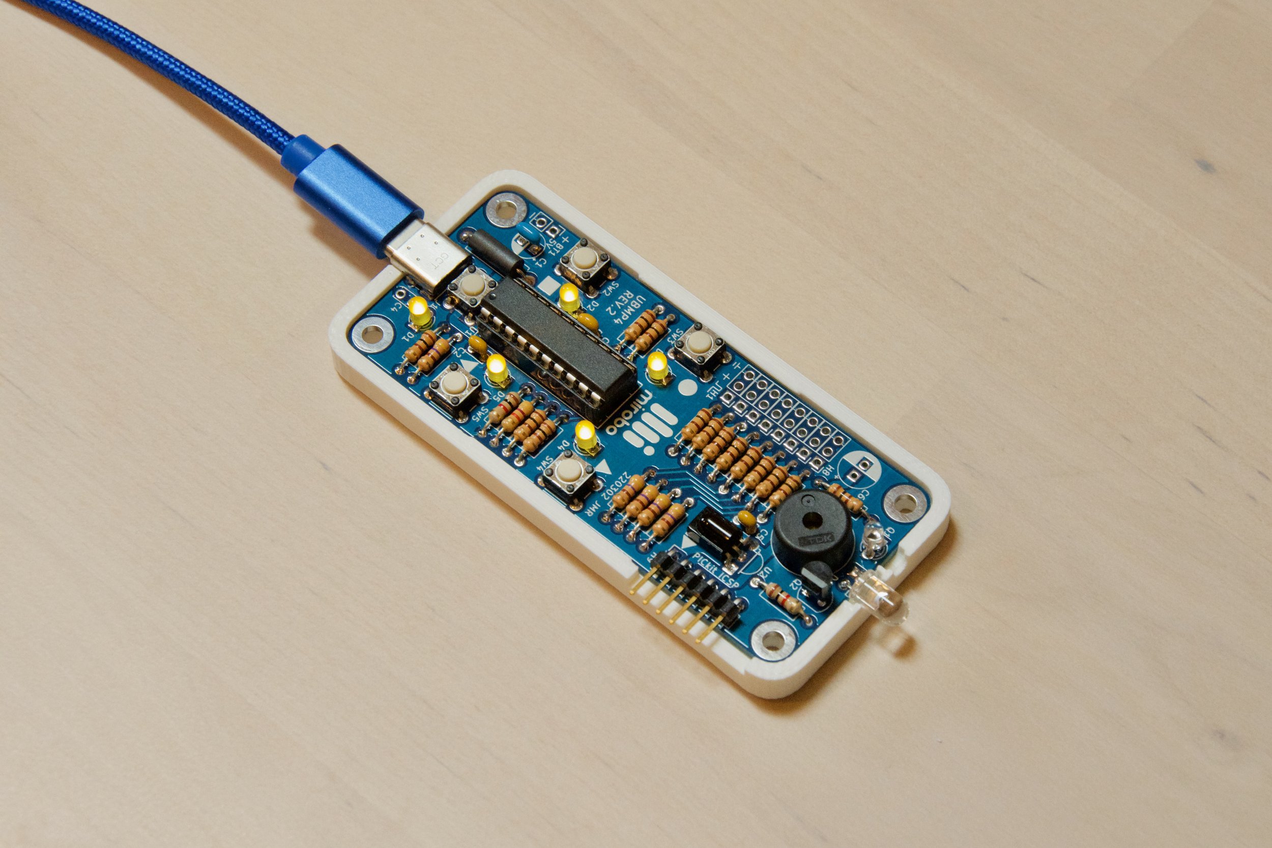
So, an LED can rapidly be flashed on and off to modulate zero and one data signals into a pulsed light beam. And a specialized demodulator circuit can be used to decode the flashing light beam and detect the ones and zeros. Both and infrared LED and a demodulator are designed into the UMBP4 circuit so it can be used to transmit and receive modulated IR codes.

The IR demodulator (circled) on a UBMP4 circuit board. The IR LED that will be used to modulate the signal is sticking out of the circuit board at the right.
Let’s explore how modulation and demodulation actually work from the transmitter and receiver’s perspective. The top signal in the diagram below consists of 40 kHz carrier pulses that rapidly turn an LED on and off. This process is one form of modulation, specifically known as frequency modulation (FM) or pulse-frequency modulation (PFM), because the 40 kHz frequency of the light pulses is the key to being able to recover information from the signal later. Modulation changes what is important about the signal: after modulation, the frequency of the group of light pulses is more important than the individual on or off states of the pulses within the carrier signal.
After being transmitted across a room these modulated LED light pulses become the input to the demodulator circuit in the receiving device, which is shown in block form below the wave:
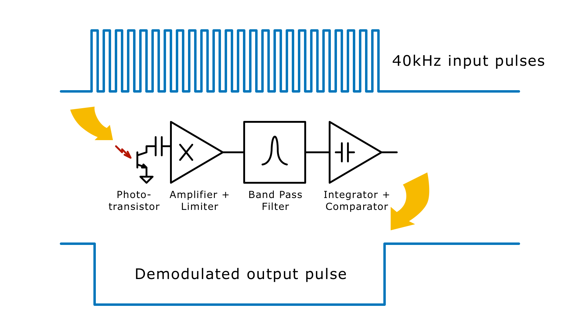
After being received by a phototransistor at the ‘front end’ of the demodulator, the flashing light pulses are amplified through a specialized amplifier and limiter circuit and then filtered through a band pass filter. The band pass filter isolates only the high frequency, flashing light signal at the frequency of interest from the continuous or slowly changing background light signal. The integrator captures this high frequency signal over time, and if the strength of the signal is above a pre-set threshold level, the comparator changes its output to indicate that a modulated signal of interest has been received. In most cases, the demodulator’s output is low when the correct frequency of flashing pulses is received, and high when no signal of interest is detected.
Data encoding
Being able to modulate and demodulate the carrier is an important first step. The next step is being able to change the modulated signal in a way that can encode the ones and zeros of our digital data. Some systems, like early modems, used two different carrier frequencies for the ones and zeros, but to keep things simple (and cheap!) IR demodulators only respond to one frequency of light pulses. A simple method of encoding data data with just one carrier frequency relies on time, namely changing the length of time that the pulses are on or off.
If the length of time that the carrier remains on is varied to make longer or shorter output pulses, this becomes known as pulse-width encoding, or pulse-width modulation (PWM). Or, if the opposite approach is taken, using the exact same length of pulses but varying time between groups of pulses, this is known as pulse-distance encoding, or pulse-distant modulation (PDM). Other encoding schemes such as Manchester (or bi-phase) encoding exist as well, but the first two are intuitively simpler to identify and decode, and they are the ones this activity will focus on.
TV and device manufacturers use all three encoding schemes. Check out the excellent SB-Projects website for a detailed description of many different kinds of IR encoding, or this Technoblogy post describing the format of the most common IR protocols. For this project, we will be exploring the comparatively simple SONY IR Command (SIRC) code. Understanding how SIRC code is encoded will provide more than enough knowledge for you to be able to modify your program to produce any other data encoding schemes later.
SIRC bit encoding
SONY uses 40 kHz carrier pulses and encodes bits using pulse-width encoding. Instead of only encoding zero-bits and one-bits, many IR protocols also encode a special start bit which is used by the demodulator to optimize its amplifier gain through a process known as automatic gain control (shortened to AGC – you might see this discussed in demodulator data sheets). SONY’s protocol encodes the following three types of bits: a long Start bit, a one bit (half the length of the Start bit), and a zero bit (half the length of the one bit). The three types of encoded bits are illustrated, below:

The pulse-width encoding is clearly visible because each bit consists of a group of a different number of identical frequency pulses, followed by the same length of space during which no pulses are transmitted. You can imagine that the transmitted signals above will produce three different lengths of lows when demodulated, separated by the same short lengths of a high signal.
To transmit each of these bits, we will need to create a program to flash an LED on and off a specific number of times. This should be easy, since it can be done using a loop, some output statements, and some time delays – all things that were covered in the introductory activities.
Thinking ahead, it probably also makes sense to create this code as a function that can be called to make each specific kind of bit. This will help to avoid duplication of the code needed to make the three different bits, and the function can be made flexible enough to allow it to be used to make any number of pulses required for transmitting data using other protocols as well.
Before we get coding, we need to figure out how to make the 40 kHz pulses. Time for a bit of math:

If the pulse frequency is 40 kHz, this means that our code has to create 40,000 pulses per second. Dividing one second by 40,000 pulses tells us that a single pulse has a period of 25 µs (microseconds). This 25 µs pulse period consists of both the high time, when the LED will be on, and the low time, when the LED will be off.
Since MPLAB has a time delay function that works in whole microseconds, let’s use 12 µs for the high time, and 13 µs for the low time of each pulse. The on/off ratio does not have to be equal – in many applications the on time is actually reduced to about 1/4 of the period to save power, and you will be able to adjust these parameters later.
Starting the program
The easiest way to start this program is to clone the UBMP4.2 Starter-1 project on Github, or download the source files. We’ll break the program into parts to demonstrate all of the coding and debugging steps for this project. The program in Github contains both the starter code, and a final version – you will learn a lot more if you follow along as the creation the final version is accomplished step-by-step from the starter code. If you are not using UBMP4, or if you want to add TV remote functionality to an existing UBMP4 program, start by creating the ir_pulse_40k( ) function, below, in your program:
void ir_pulse_40k(unsigned int pulses) // Makes requested number of 40kHz pulses
{
    for (pulses; pulses != 0; pulses--) {
        IRLED = 1;              // Create 25us period waves
        __delay_us(12);         // Use 12us on and 13us off for ~50% duty cycle
        IRLED = 0;              // (25% duty cycle can be used to save power)
        __delay_us(13);
    }
}
This function definition specifies an integer variable for the number of pulses it will make because some protocols require more than 256 pulses to create their really lengthy start bits. The SIRC protocol could make do with an 8-bit character variable, but using a 16-bit int variable allows this function to be more versatile. The rest of the code seems fairly straightforward, with a for loop to count down the number of pulses remaining and instructions inside the loop to turn on the LED, wait the required number of microseconds, turn off the LED, and wait again before beginning the next pulse.
We can test this new function by calling it with a number from the main code. We could use any number for testing, but why not use the number of pulses for one of the bits that will need to be encoded? Let’s perhaps use the number of pulses required for the start bit. In the SIRC protocol, the start bit is 2.4 ms long , and the 40 kHz pulse period is 25 µs, so the number of pulses needed for the start bit can be determined by dividing:
2.4 ms / 25 µs = 96 pulses
96 pulses will provide ample opportunity to take measurements of the individual pulses and the length of the group of pulses using an oscilloscope. To make testing easier it’s often helpful to add a delay between groups of pulses to clearly mark the start and end of each group as well as to provide another signal (a long low period, followed by pulses) for the oscilloscope to trigger on.
The main( ) function in the program starts with the typical UBMP4 configuration code and then adds the pulse function and a delay to the main while( ) loop. The if(SW1 == 0) condition is used by UBMP4 to re-start its bootloader. This code is all that will be needed to test the pulse function:
int main(void)
{
    OSC_config();               // Configure internal oscillator for 48 MHz
    UBMP4_config();             // Configure on-board UBMP4 I/O devices

    while(1)
    {
        ir_pulse_40k(96);       // Pulse test code
        __delay_ms(15);         // Delay between pulses

        // Activate bootloader if SW1 is pressed.
        if(SW1 == 0)
        {
            RESET();
        }
    }
}
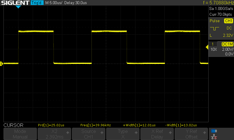
The next step is to test the program to confirm that it actually generates 96 accurate pulses. Here is the result:
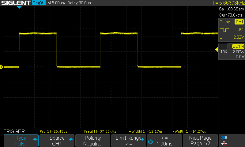
The measurements below the wave show that the expected 25 µs pulse is a bit too long…
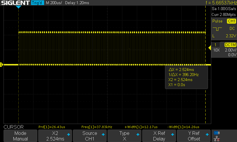
As a result, the start bit of composed of 96 pulses is also longer than the 2.4ms expected.
Debugging the code
Oh no, the pulse timing is off, although it is close to the target values. What do you think happened to cause the inaccuracy?
One of the first challenges programmers face when writing hardware timing programs is understanding that all of the program code itself takes time to run. How much time each part of the code takes to run is more difficult to comprehend when programming in C code as compared to assembly code, as C language statements do not translate directly to machine code instructions as assembly statements would. Programmers writing in assembly code will have a much better idea of how long each part of their code will take to run, but assembly code is more challenging to write, and requires a deeper hardware understanding of the microcontroller than C. So, as C programmers, we have to use our test equipment and intuition to figure out what is causing the delays in our program.
Using the oscilloscope to capture of the output signal, we can get a good idea of where the delays take place. From the measurements shown at the bottom of the oscilloscope screen, the high part of each pulse is 12.17 µs, which is very close to the 12 µs delay specified in the code. The low part, however, is 14.26 µs instead of the expected 13 µs. Something related to this part of the program is taking too long. But what? Can you figure it out from the code reproduced below?
    for (pulses; pulses != 0; pulses--) {
        IRLED = 1;              // Create 25us period waves
        __delay_us(12);         // Use 12us on and 13us off for ~50% duty cycle
        IRLED = 0;              // (25% duty cycle can be used to save power)
        __delay_us(13);
    }
The answer may not be immediately obvious to anyone new to programming microcontrollers, or to programmers whose only experience is writing code for fast, desktop microprocessors. They delay is actually caused by the for( ) loop. How can we tell? The for loop updates its count after the LED is turned off, extending the time that the LED is off, and before it turns on again. But, why would a for loop take so long? Isn’t the for loop just updating a counter variable?
To get a better understanding of why the for loop takes so long, its operation has to be broken down into its individual, machine code steps. Each step takes one or more microcontroller instruction clock cycles, and each microcontroller instruction cycle in this case will be 83.3 ns in length. How do we know? To calculate the instruction clock cycle time for any mid-range PICmicro device, divide the master clock frequency by 4 (so 48 MHz / 4 = 12 MHz) to get the instruction frequency, and then take the reciprocal of the instruction frequency (1 / 12 MHz = 83.3 ns) to find the instruction cycle time period. The more program steps there are in a function, the more time the function will take, adding more delay.
Understanding the machine code
The following pseudo-instructions illustrate the typical sequence of machine code instructions that would make up the for loop, including everything that happens between the end of the 13 µs delay until the point that IRLED is turned on again. These steps should exactly correspond to the length of the low, or off time, of the wave. Listed in the brackets are the number of instruction cycles each step could take. An instruction cycle is the time taken to complete one, simple instruction. Complex instructions can take more time to complete. Brackets showing two numbers show the number of instruction cycles for a branch not taken (the first number), or for a branch taken (the second number) by the microprocessor. If a branch is not taken, the next instruction below it is executed, typically resulting in two successive single-cycle operations, whereas if a branch is taken the next instruction is skipped resulting in a single, two-cycle operation – since both are two cycles, the branch decision won’t affect the loop’s overall execution time. Here is the pseudo-code equivalent of the for loop:
jump to the start of the for loop                      (2)
subtract 1 from the low byte of pulses                 (1)
check for a negative result and skip if positive       (1 or 2)
subtract 1 from the high byte of pulses                (1)
check the high byte of pulses for 0 and skip if 0      (1 or 2)
jump to LED_ON                                         (2)
check the low byte of pulses for 0 and skip if 0       (1 or 2)
jump to LED_ON                                         (2)
exit
LED_ON - turn IR LED on                                (2)
Adding up the pseudo-code clock cycles, the for loop will take 13 instruction cycles to complete. The amount of time these cycles add to our function can be calculated by multiplying the instruction cycles by the instruction clock time:
13 * 83.3 ns = 1.083 µs
How does this guess, using pseudo-instructions, match the real result? Recall that the program code calls for a 13 µs delay after turning IRLED off. After that, the for loop will add its 1.083 µs to the 13 µs delay, for a predicted total of 14.083 ms before IRLED is turned on again.
From the oscilloscope capture, the actual off time was measured as14.26 µs – so the calculation was pretty close. Not exact, but at least now we have an understanding of the source of the error in our pulse timing code, and we can explore different ways to fix it. The first method involves the use of the built-in MPLAB X code simulator which can eliminate the need to have an oscilloscope for debugging.
MPLAB X Simulator
The MPLAB X IDE includes a simulator that allows users to debug their code without running the program in any hardware. Obviously, not all code can be simulated, especially if the code needs to interact with hardware devices. But, the simulator can be incredibly useful at finding code path and timing issues in user programs. Running code in the simulator is almost as easy as just compiling the program. First, the simulator has to be enabled for the project, and the simulation clock speed has to be set to match the target device.
Enable and set up the simulator
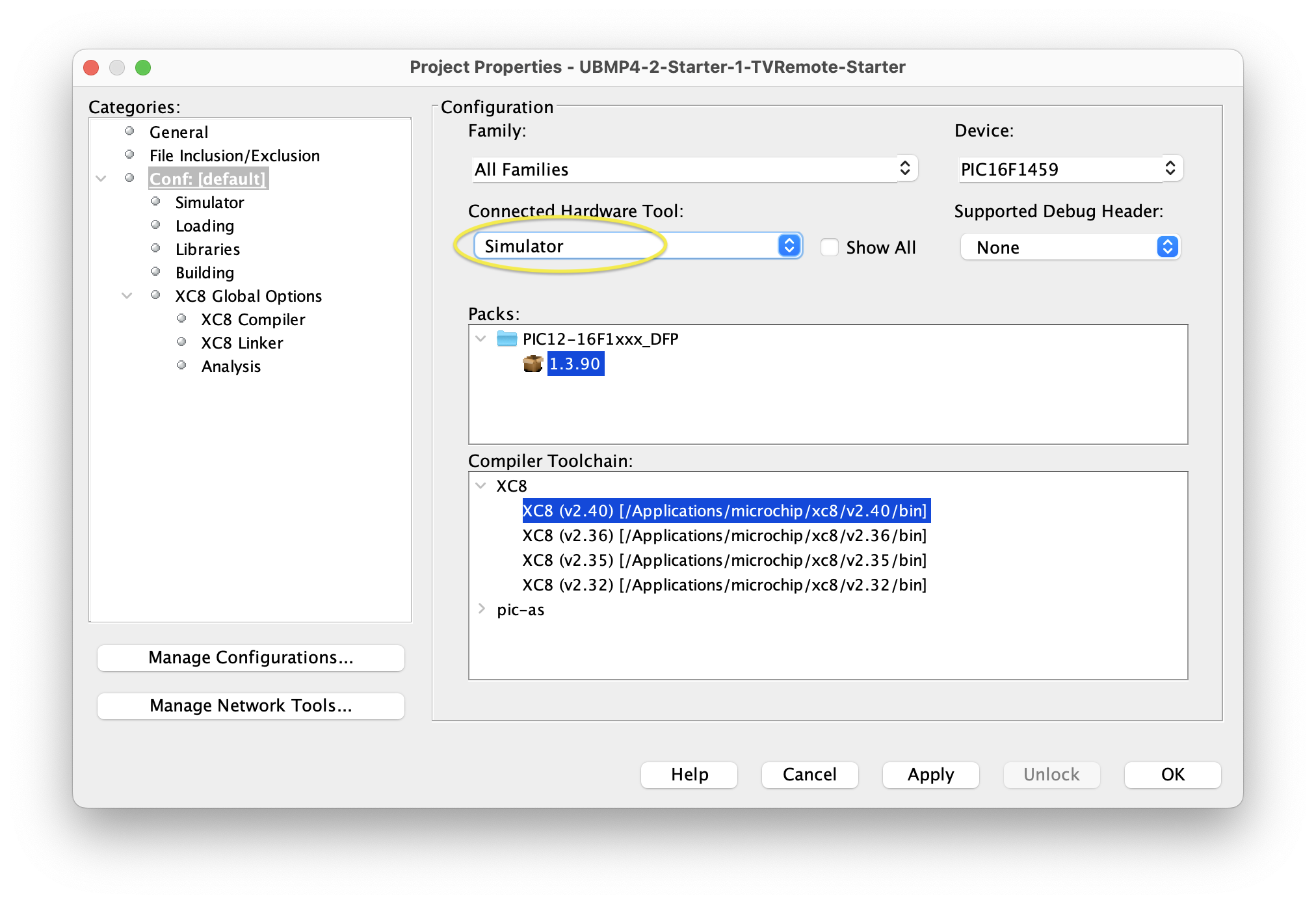
To enable the simulator, click on the Project Properties button (the wrench and gears) in the Dashboard window at the lower left of the MPLAB X screen. In the project properties window, set the Connected Hardware Tool to Simulator, and click the Apply button to apply the setting without closing the window.
Next, click on Simulator in the Categories pane at the left to open the Simulator Options panel. In the Simulator Options panel, under the Oscillator Options pull-down, set the Instruction Frequency to 12 MHz. This allows the simulator to time the code execution properly for the 48 MHz oscillator clock rate of the PIC16F1459 microcontroller used in UMBP4. Click OK to save the settings.

Start the simulation
Next, start the simulation by clicking the Debug Main Project button in the MPLAB X toolbar. The simulator/debugging toolbar opens up at the top of the screen to reveal the additional debugging control buttons shown here:
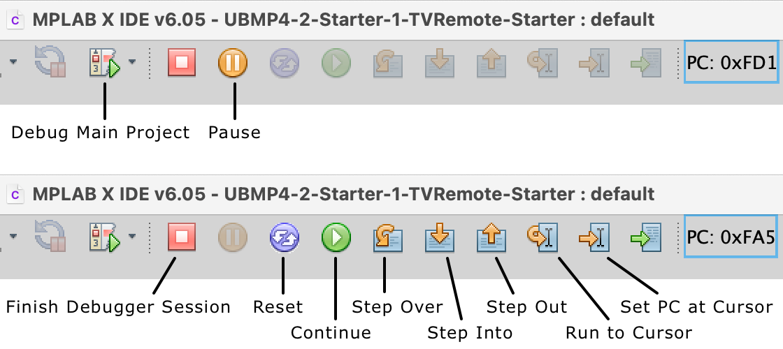
The top bar shows the simulator/debugging toolbar when the program is running. Additional features are enabled when the program is paused as shown in the bottom bar.
After pressing the Debug Main Project button, the MPLAB X re-compiles the program for simulation and begins running the program. Oddly, it won’t look like anything at all is happening on screen. While the simulation is actually running, it is not running in an interactive way, yet.
Press the Pause button on the debug toolbar at the top of the windows to stop the simulation. A highlighted code line will indicate the current location of the program counter in the editor window, showing the instruction – technically the C statement containing one or more machine code instructions – that is about to be simulated. The program seems to have stopped at the while(!PLLRDY); statement in the UBMP420.c file. Why is that?
The microcontroller’s PLLRDY (phase-locked loop ready) flag will be set when the hardware PLL is stable, but unfortunately this flag is not modified by the simulator. So, simulation is stopped here as the simulator is waiting for a bit that never changes. Frustratingly, there is no error message or notification that simulation has abruptly come to a halt, only us pausing the simulator gave us a clue that we encountered a problem. Using the simulator for more projects you will occasionally encounter other similar, silent failures. Despite all that, once a work-around is found, simulation can still be an incredibly helpful tool.

To bypass the stalled code and continue the simulation, add two slashes // to comment out the entire line containing the while statement in the OSC_config( ) function. Note that the code comment at the end of this line in the program also indicates that this line must be disabled for simulation. Remember to re-enable this statement in the code by removing the slashes after the simulation session is finished!
Restarting the simulator
The debugger needs to be exited and restarted after any code changes have been made, and commenting out an instruction is definitely a significant code change. Press the Finish Debugger Session button to exit the simulator. Ensure that the while(!PLLRDY); statement is commented out (it will be grey, instead of black, in the code editor), and press the Debug Main Project button to start the simulator again. MPLAB X will re-compile the modified program and the simulator will begin to run it again. And, once again, after the simulator start it will still look like nothing is happening.
Press the Pause button to stop the simulation. The first clue that the program is now actually running and being simulated is that the highlighted line showing where the program halted will be at a different location in the code editor than before.
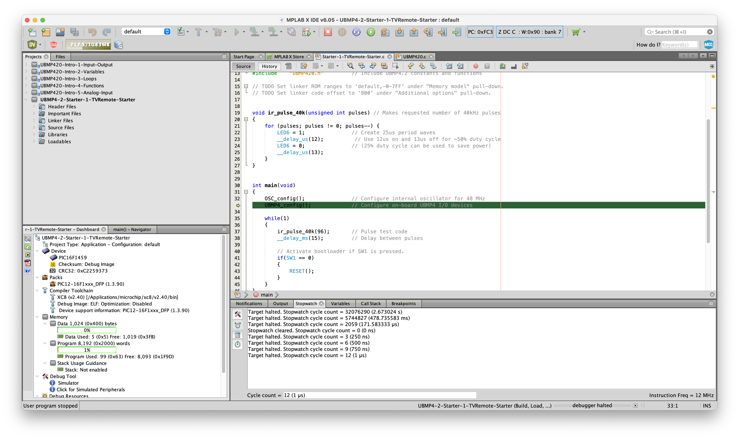
The program was running, invisibly doing things, until it was paused. We didn’t know which code was run, or in what order, or how many times it ran. To actually see what is really happening in the program, it has to be re-started from its start-up state. Press the Reset button (the purple one with the two circular arrows) in the debugging toolbar to reset the microcontroller’s program counter to the start of the program. The program counter should be stopped on the first line in the main( ) function, as indicated by the highlighted line in the code, below:

Enable the Stopwatch and step through the code
The debugger contains a stopwatch tool that can be used to evaluate the program’s instruction cycle timing and loop timing. From the MPLAB X Window menu, choose Debugging and then choose Stopwatch from the secondary window.


Click the Stopwatch tab in the lower panel below the code editor to open the Stopwatch output panel. Press the bottom icon at the left of the Stopwatch panel to clear the stopwatch – the icon looks like a stopwatch that’s ready to start timing!

Your stopwatch may show a different number of counts than in the screenshot above, but the bottom statement in the Stopwatch panel is the most recent stopwatch value and should show a count of zero clock cycles and zero nanoseconds (ns) after being reset.
Start single-stepping into the code by pressing the Step Into button (vertical arrow down) on the toolbar once. After this first press, the highlighted code cursor jumps into the code of the OSC_config( ) function in the UBMP420.c file which, if it was not open before, will now be open in the code editor.

In the example above, the microcontroller has taken 3 instruction clock cycles to get to this next program instruction, or 250 ns at the microcontroller’s 12 MHz clock frequency (the instruction frequency is also indicated at the bottom right of the window). The currently highlighted line of code in the program has not yet been run – the highlight shows the position of the microcontroller’s program counter, which is the position corresponding to the instructions in code that will be run next.
Press the Step Into button again. The highlight will move down one line, and the Stopwatch will update the cycle count and run time.
Press Step Into again. Why is the closing brace } highlighted? It can’t be run, it’s not an instruction! The simulator is trying to show the position of the program counter, and the counter has moved beyond the ACTCON = 0x90; statement, or whatever its equivalent machine code statements – plural, because they seem to take more than one cycle – are. In this case, the program counter is likely at the machine language return statement, used to return from a function call. Since there is not a one-to-one relationship between C and machine code, and the return is assumed to take place at the end of the function, the highlighted-line program counter display can often end up in what looks like a strange place in the C code. This is normal, and usually happens at the beginning or end of a function, or in conditional statements.
Press Step Into once more to exit the function and return to the next line of the main( ) program.
The Stopwatch shows that running all of the steps in the OSC_config( ) function took 12 clock cycles, or 1 µs of program time, and each of the individual steps is clearly listed since we chose to step through the code line-by-line. You can imagine that stepping through an entire program like this would get tedious, especially for long loops within functions.
Rather that stepping through each of the parts of the UBMP4_config( ) function, there is a shortcut that can be used to bypass all of the unimportant (for us) code in the simulator. Press the Step Over button (curvy arrow down) to have the simulator run through the next instruction’s code – in this case all of the code in the next function call – invisibly, and then stop the program counter at the next statement in the code.

That was easy! With one click, another 23 instruction cycles flew by! If you accidentally clicked the Step Into button and ended up inside the UBMP4_config( ) function in the simulator, just click the Step Out button (vertical up arrow) to get out. Or, not. You might actually want to step through the UBMP4_config( ) function if you are interested in seeing what happens in it. It’s up to you!
When there are successive program statements, and not functions to run, the Step Over button acts like the Step Into button, so it’s easy to just keep clicking on the Step Over button to avoid accidentally stepping into functions and loop code.
Timing the pulses in the simulator
Keep clicking the Step Over button until you end up at the IRLED = 1; statement in the ir_pulse_40k( ) function. To measure the on time of the LED, we have to either memorize the stopwatch count or, even easier, reset the stopwatch and use it to do the timing. Click the Clear Stopwatch button to reset the count. Then, Step Over the statement to turn the LED on, as well as the 12 µs delay function call.

After clearing the stopwatch, we can see that it took 2 instruction cycles to turn on the LED, and the equivalent of 144 cycles to delay by 12 µs, or a total of 146 cycles from when the stopwatch was reset. This total on-time is very close to the target 12 µs on-time value we were trying to achieve.
Clear the stopwatch again, and press the Step Over button until the IRLED = 1; statement is highlighted to simulate the off-time of the loop.

Each press of the Step Over button step adds another time record to the Stopwatch panel output list. We can see it takes two cycles to turn IRLED off, then 13 µs were added by the delay function to increase the total cycle count to 158. Following that is an increase of six cycles, and then another increase of 7 cycles, before the code simulator lands back at the starting point where IRLED was first turned on. From our previous exploration of the machine code, above, we have an understanding of what causes this extra delay – the code counting down in the for( ) loop. Even if, as a new programmer, you have a very limited understanding of machine code, the stopwatch and simulator clearly show that there is a timing delay in this part of the code. You may not understand the cause of the problem, but you do now know the location to focus code changes on in order to fix it.
Oh, and did you notice that the total times for the LED on and off periods calculated by the simulator exactly match the timing of the wave originally measured using the oscilloscope! This fact makes the simulator an accurate option for calculating code delays before testing actual hardware, and may eliminate trial and error testing alternating between code changes and measurements using test equipment.
Run to here
Here is one last simulator tip to quickly jump to a section of interest. Position the cursor over the line of code containing the statement IRLED = 1; and then right-click the mouse button. Choose Run to Cursor from the pop-up menu that appears to set the simulation program counter to this exact line of code.

Next, reset the Stopwatch by pressing the clear button, and then again position the cursor over the same line of code containing IRLED = 1;. Right-click and choose Run to Cursor again. The simulator has now run one complete cycle of the entire ir_pulse_40k( ) loop from when the stopwatch was reset, and the Stopwatch output panel will show the total time taken by all of the code running through one complete for loop.
The Run to Cursor function works great after re-starting the simulator, too. This is especially useful when making code changes while debugging code. After re-starting the simulator, press the simulator Reset button, then hover the cursor over the code of interest, right click, and choose Run to Cursor from the pop-up menu. Voila, the simulator is stopped at exactly the section of code you want to test!
This is just a short introduction to one way in which the simulator can be used in code debugging. The simulator includes other useful features for developing and debugging code, but these main button controls are all that we will explore in this activity.
Fixing the pulse timing
So now both the oscilloscope measurements have shown that the low part of the pulse is too long, and the simulator has confirmed that extra code is running during the low part of the pulse. Since we can’t change the for loop, perhaps the low part of the pulse can be shortened by decreasing the delay in the code? After the line that turns IRLED off, try changing the delay to 12 µs (from the original 13) and then test the program using either the simulator or an oscilloscope. What happens?
Decreasing the delay by one microsecond in the code should have had the exact same effect on the output pulse. One complete pulse will now be exactly one microsecond shorter, or 25.42 µs, but still longer than the 25 µs we were trying to achieve. Decreasing the time delay by another microsecond in the code shortens the output pulse to 24.42 µs – again exactly one microsecond shorter than before. Is that the minimum length of time that the code can be changed by? It’s close, but it seem we will not be able to achieve an exact 25 µs pulse period if the code can only be changed in one microsecond intervals.

There are at least of couple of methods of tweaking the code delay: one is a poor choice for this example, and another is a much better choice. The poor choice involves the addition of NOP(); (no operation, or no-op) instructions to add extra instruction cycles of execution without affecting any other part of the program. No-ops add time but also take up program memory space, and can be a viable alternative when just one or two carefully-placed clock-cycle delays can tweak or equalize the timing of a section of code. Fixing this code with no-ops, however, would require too many and would also be an inelegant solution.
In this case, the preferred method of fixing the timing is to replace the microsecond delay function with a clock cycle delay function. Microchip provides a number of different delay functions, described in the compiler help documentation, that can be used to get code timing just right. Again, as we substitute delay functions, the simulator can be a great help to get the timing exactly right with the minimum trial and error code modifications.
Looking at the prior runs, the clock cycle count to both turn IRLED on and perform the 12 µs delay was slightly too long at 146 cycles. This was just two instruction cycles longer than the 12 µs we wanted. What if we could just subtract the two extra cycles from the delay, making the delay 142 cycles long instead of 144? And, following the same logic, can the off pulse delay be shortened to subtract out the clock cycles taken by both the return instruction and the instructions in the for( ) loop? It turns out we can do just that. Here is the modified delay code using the clock cycle delay functions:
    for (pulses; pulses != 0; pulses--) {
        IRLED = 1;              // Create 25us period waves
        _delay(142);            // Use 12us on and 13us off for ~50% duty cycle
        IRLED = 0;              // (25% duty cycle can be used to save power)
        _delay(141);
    }
The original __delay_us( ); functions have been replaced by _delay( ); clock cycle delay functions. Be careful, the clock cycle delay function uses a single underscore character at the beginning of its name instead of the two used by the microsecond and millisecond delay functions. These new delays will produce exactly the pulse output timing needed: 12 µs on, 13 µs off, producing a pulse period of exactly 25 µs as shown in the simulator run, below:

Finally! Exact time pulses using clock cycle delays.
Now, let’s use the oscilloscope to confirm the length of the individual pulses, as well as the total length of the Start bit composed of 96 pulses.
Each complete LED pulse is now exactly 25 µs long.

The 96-pulse Start bit is now exactly 2.4 ms long. Woohoo!
Formatting SIRC data
Now that the ir_pulse_40k( ) function in our code makes accurate 40 kHz pulses, it can be called from other functions to encode bit data. Any length of bit can be made, including bit lengths required to encode either PWM- or PDM-formatted data. Since the original goal was to make Sony IR Command (SIRC) formatted PWM data, let’s examine the simplest 12-bit SIRC data encoding protocol.
The top waveform shows the shrunken-down, 40 kHz pulse-width encoded wave that would be fed to an IR LED. Three different lengths of encoded pulses are visible, with the first three pulses in the waveform corresponding to the length of the start bit, a one bit, and a zero bit, respectively. There are a total of twelve zero or one pulses following the start bit in the 12-bit SIRC protocol.

The bottom waveform shows the pulses as they would be received by a microcontroller after being decoded by a demodulator IC. The bit data being received corresponds to the lengths of the low output periods of the received wave, and each bit value is indicated below the wave. Note that the bits are divided into two groups: seven command bits, representing the button pressed, and five device bits representing the type of device being controlled. These divisions allow a company like SONY, who make a large variety of products, to re-use the same command codes for multiple devices. For example, a TV, a DVD player, and a PlayStation can all use the same power-on command. Only the device bits of the transmitted signal would be different for these three devices.
Using seven command bits allows SIRC devices to have up to 128 functions – that remote would have a lot of buttons! The five device bits allow up to 32 different kinds of devices to be controlled. Newer SIRC procols have been updated to support eight device bits (15-bit SIRC protocol), or eight devices bits plus 5 extended attribute bits (20-bit SIRC protocol). Older and simpler devices still use the 12-bit protocol, and the 12-bit SIRC data encoding will be used as the example code for developing a TV remote control program here.
Formatting serial data
The seven command bits and five device bits can each be stored in separate bytes of data in our program. The process of formatting the serial data involves evaluating the state of each bit in the bytes, and then transmitting the right number of pulses for each bit, in the correct order and with the appropriate spaces in between them to produce the PWM-encoded data signal.
The order of the bits in a SIRC-encoded transmission is from least-significant bit (LSB) to most-significant bit (MSB). The process of evaluating each of the bits is exactly like that used in the serial output function introduced in Introductory Activity 5, namely isolating and testing the LSB, and shifting the data over one bit to move the next bit in the byte into the LSB’s position.
The difference between this code and the serial transmission program is that after evaluating a bit the serial output program encodes the state of each bit as a simple voltage on a pin, while the remote control program has to modulate the carrier with the proper number of pulses and then add a bit delay. Another difference is that this program will transmit two different sets of data – the command bits, and the device bits – in succession for each piece of coded data being sent. Other protocols, such as NEC, transmit four bytes of data for each code being sent.
Programming for flexibility and readability
Since creating different remote control data protocols relies on generating similar groups of pulses, it will be easier to adapt this code for use with other formats if the functions are made to be as flexible as possible. One way to do this is to not hard-code values into any function. Instead, the values can be defined as program constants and substituted as needed between SIRC and other data formats. Add these SIRC constant definitions at the top of the program, or open the final version of the program, with all of the upcoming changes included, from the Github project:
// Sony IR protocol definitions
#define SONY_START_PULSES   96  // Number of 38kHz IR pulses in a start bit
#define SONY_1_PULSES       48  // Number of IR pulses to encode a one bit
#define SONY_0_PULSES       24  // Number of IR pulses to encode a zero bit
#define SONY_BIT_DELAY      600 // Space between data bits in microseconds
#define SONY_COMMAND_BITS   7   // Number of command (data) bits to be sent
#define SONY_DEVICE_BITS    5   // Number of device (address) bits to be sent
The constant names are defined in upper case letters to match Microchip’s conventions found in MPLAB and other hardware programming conventions. Having all constants in capitals is not a requirement, but it is a visual clue that these are not variables so it can help a programmer to recognize that they can only be changed by modifying their definition statements. To be totally clear about the intention their use, each definition name is prefaced by its target device (SONY in this case), so that what the code is trying to accomplish becomes more obvious to anyone reading it. For example, creating a start pulse for the SIRC protocol like this…
    ir_pulse_40k(SONY_START_PULSES);
    __delay_us(SONY_BIT_DELAY);
…is more readable and meaningful than this:
    pulse(96);
    __delay_us(600);
Both sets of code would accomplish the same thing (assuming the pulse( ) function was the same as the ir_pulse_40k( ) function), but the top example provides more information about what the function does, what data it is being sent, and the meaning of the data. And, if we wanted to use the same pulse function to make different lengths of start pulses for different protocols, we would need two different definitions anyway, so adding SONY_ to the name makes it perfectly clear which start pulse it is.
SIRC transmit function
Transmitting data using the SIRC protocol involves three steps: making a start bit, transmitting seven command bits in LSB-first order, and finally transmitting five device bits in LSB-first order. Using the descriptively-named constants defined above, here is a complete function to transmit the 12-bit SIRC code:
void ir_transmit_Sony(unsigned char device, unsigned char command)
{
    // Create Start bit followed by bit delay
    ir_pulse_40k(SONY_START_PULSES);
    __delay_us(SONY_BIT_DELAY);

    // Transmit command bits with bit delays
    for (unsigned char i = SONY_COMMAND_BITS; i != 0; i--)
    {
        if ((command & 0b00000001) == 1)  // Isolate LSB to determine its state
            ir_pulse_40k(SONY_1_PULSES);
        else
            ir_pulse_40k(SONY_0_PULSES);

        command = command >> 1; // Shift next bit into position
        __delay_us(SONY_BIT_DELAY);
    }

    // Transmit device bits with bit delays
    for (unsigned char i = SONY_DEVICE_BITS; i != 0; i--)
    {
        if ((device & 0b00000001) == 1)  // Isolate LSB to determine its state
            ir_pulse_40k(SONY_1_PULSES);
        else
            ir_pulse_40k(SONY_0_PULSES);

        device = device >> 1;   // Shift next bit into position
        __delay_us(SONY_BIT_DELAY);
    }
}
Transmitting data
The function call statement shows that the transmit function requires two pieces of data, representing the device code and command. We could just make up any two pieces of data to test with, but using real data will make it easier to verify that the function actually works as planned. To obtain real data, an oscilloscope was used to capture and decode the most useful command codes transmitted by a SONY TV remote, and this data was used to generate the following list of constant definitions:
// Sony IR command (data) codes
#define SONY_CH1    0x00        // Channel number button codes
#define SONY_CH2    0x01
#define	SONY_CH3    0x02
#define	SONY_CH4    0x03
#define	SONY_CH5    0x04
#define	SONY_CH6    0x05
#define	SONY_CH7    0x06
#define	SONY_CH8    0x07
#define	SONY_CH9    0x08
#define	SONY_CH0    0x09

#define	SONY_CHUP   0x10        // Channel up button code
#define	SONY_CHDN   0x11        // Channel down button code
#define SONY_VOLUP  0x12        // Volume up button code
#define	SONY_VOLDN  0x13        // Volume down buttoncode
#define	SONY_MUTE   0x14        // Mute button code
#define SONY_POWER  0x15        // Power on/off button code

#define	SONY_INPUT	0x25        // Input select button code

// Sony IR device (address) codes
#define SONY_TV     0x01        // TV device code
Controlling a SONY television will now be as easy as calling the transmit function with the TV device code followed by the command code. For example, to turn the TV on (or off – it’s the same code) we could write the following statement into our program:
ir_transmit_Sony(SONY_TV, SONY_POWER);
If you happen to have a SONY television and you try this code in your UBMP4 to transmit one, single power command to your TV, you will find that it unfortunately does not work to turn on the TV. The code works, making the encoded data, and we are actually so close to having success. There is just one more thing you need to know that relates back to the introduction to encoding data with light at the top of this page, including the unreliability of a room with a dog (remember the dog?) as a medium for a data signal. And, unfortunately, this part is not something that can be simulated, although an oscilloscope would provide the final clues needed to make the transmission work.
Error checking, key repeat rate, and data frames
Assuming something will go wrong allows that possibility to be planned for, including planning ways to mitigate the problem. The engineers who created these remote control protocols understood that errors could be introduced in the signal and devised various solutions to ensure the reliable transmission and reception of data. To be clear, receiving data without errors is the really hard part – we have the much easier task in this program of simply transmitting the data. But, we still need to understand how a receiver might deal with error checking because that will affect how, and how many times, the data has to be transmitted.
Let’s examine what could go wrong while transmitting bits using the SIRC protocol. First, another light source in the room could mimic the 40 kHz carrier wave signal. Sunlight is essentially unchanging, and standard room lights operate at 50 or 60 Hz, so neither of those should be a concern, but some high efficiency fluorescent and some LED lights can pulse at various multi-kHz frequencies and could be picked up by the demodulator. In this case, this high frequency light would have the effect of lengthening the demodulated pulses, potentially changing a zero bit to a one bit. More likely, any significant increase in the length of the pulses will interfere with the bit timing enough to make the data indecipherable to the receiver, and the receiving program will ignore the data.
More likely than the first possibility is that a weak signal or long range makes it more difficult for the received light signal to exceed the demodulator’s internal threshold, shortening or eliminating some data pulses. This could potentially change a one bit to a zero bit in the transmission though, as before, if enough bits are affected or the spaces between the bits are too long, the receiver software should ignore the data if it is too different from the protocol.
The last possibility is that you and another member of your household are fighting for control of the TV by each having your own remote and pressing buttons at the same time, but that error mode is a human problem that the two of you will have to work out, rather than a technical problem with the protocol. Wait, we are actually building a program to make UBMP4 into another remote transmitter though, aren’t we? So, yes, this could also become a potential problem.
To deal with some occasional interference that might stretch a zero bit to a one bit, or shrink a one bit to a zero bit, the creators of the SIRC protocol opted for their error checking to require the receiver to recieve two identical pulses in a row, and to receive both of these pulses within a specified time period. Assuming the first data transmission is correctly received and the second is garbled in some way, the receiver will not know which of the two is correct and will choose to wait and do nothing. When the third transmission is received without error, it will not match the second, so the receiver will still wait and do nothing. When a fourth transmission is received, and the fourth transmission matches the third, the receiver will act perform that action called for by that command. The likelihood of two commands becoming garbled in the exact same way by interference is so low that receiving two identical codes in a row confirms that they were correctly received.
Now, you should understand why sending just a single SIRC transmission would not turn the TV on. The TV needs to receive two identical power command transmissions in a row before it will turn on. But, if one of the transmissions is received as damaged, at least one, or maybe two more need to be sent. So, it makes sense to transmit the same data repeatedly, in the hopes that the receiver will detect two identical codes in sequence.
In the SIRC protocol, the same data is repeatedly transmitted while a key is pressed. Some other protocols implement a special repeat code instead of repeating the same command code. It’s up to the receiver to decide what to do with repeated codes. For example, it makes sense for a TV to keep increasing its volume while the volume up command is repeated if the volume button is held, but it would be annoying if the TV kept turning on and off whenever the power button is held.
The repeat rate of the data transmission could be used by the receiver to set the rate of a volume change, for example, or the receiver could implement its own volume adjustment rate to make it independent of any received data errors. Also, the receiver should clear its data if too much time passes so it doesn't match a newly received piece of data with and old stale one.

The SIRC data frame repeats every 45 ms, from the start bit of the first transmission to the start bit of the following transmission. This value does not have to be that exact, but too long or too short might result in it being discarded by the receiver. Because it is difficult to time from the beginning of one transmission to the next, we will cheat and just add a partial frame delay in between transmissions.
Here, finally, is the main code to turn a SONY television on (or off) whenever pushbutton SW3 on UBMP4 is pressed:
int main(void)
{
    OSC_config();               // Configure internal oscillator for 48 MHz
    UBMP4_config();             // Configure on-board UBMP4 I/O devices

    while(1)
    {
        if(SW3 == 0)
        {
            ir_transmit_Sony(SONY_TV, SONY_POWER);
        }

        // Data frame delay between button presses (adjust based on protocol)
        __delay_ms(25);

        // Activate bootloader if SW1 is pressed.
        if(SW1 == 0)
        {
            RESET();
        }
    }
}
Next, let’s test the code using the oscilloscope. Here is a capture of one and a half complete data frames:

Two successive frames of a SONY TV power command, showing one complete encoded data frame and gap, and just the encoded data frame.
Zooming in, we can get a close-up view of the PWM-encoded data bits in the data frame.

A single power command, clearly showing the different lengths of the start bit, and the zero and one bits.
We did it! You now have a new way to turn any SONY television on and off. If you don’t have a SONY TV, this code won’t be as quite as useful for you as it is for me (I happen to have two). If it’s any consolation, you have now seen how easy the SONY SIRC protocol is to produce because of its simplicity, and this simplicity means that it is also fairly easy to decode (and, as a result, to implement in your own circuits). And, after following along all the way through this activity, you should have a much better understanding of remote control protocols and a good framework for structuring your program code to encode IR data in any protocol. Hopefully, you will also have a developed a basic understanding of how to use the built-in MPLAB X simulator, and can use it to help debug and optimize your program code and time delays in future projects.
TV remote learning summary
Infrared remote control transmission relies on modulated carrier pulses of a specific frequency that can be decoded by specialized demodulator circuits. Groups of these carrier pulses can be encoded in different ways – pulse-width (PWM), pulse-distance (PDM), and bi-phase – to represent data. Data transmission as light pulses through the air is inherently unreliable, so other techniques must be used to ensure the data is received properly, including sending multiple, identical transmissions to a receiver.
Microcontrollers are fast, but executing multiple instructions takes some amount of time. When programming a microcontroller to generate high frequency pulses, the time taken by the instructions running the code can add a significant amount of extra delay between the pulses, affecting the timing. This extra time must be accounted for, usually by shortening delays between the pulses.
The use of a code simulator to investigate instruction flow within a function, or the use of an oscilloscope to analyze software output are both useful tools when predicting and adjusting software timing in critical time delay code.
TV remote programming challenges
Not all IR protocols encode data using a 40kHz carrier. The NEC protocol uses a 38kHz carrier, and the Philips RC-6 protocol uses a 36kHz carrier. Create and debug a pulse function to produce modulated pulses at one of these other frequencies.
The NEC protocol (or a slight modification of it) is used by many brands of televisions including LG and Samsung. Research the NEC protocol. What type of modulation is used to encode its data?
Determine the number of pulses required to create a start bit, a zero bit, and a one bit for the NEC protocol using a 38kHz carrier.
You can clip an oscilloscope lead to the output pin of the UBMP4 IR demodulator (U2) to view remote control pulses from many remote control transmitters without needing to write any software code. See if you can decode and reverse engineer the IR protocol transmitted by a remote control transmitter that you own or have access to.
Create a flowchart of the software functions that would be needed to transmit a protocol different from the SIRC protocol.
IR protocols can be created to implement your own controllable devices. Think about the types of commands you would need to encode to remotely control a robot, or a string of NeoPixel LEDs.